Runing Pandeia TSO from the terminal
This Python script shows how to run TSO simulations with Gen TSO from an interactive Python session
Setup target
Lets set the target properties first:
import gen_tso.pandeia_io as jwst
import gen_tso.catalogs as cat

import numpy as np
import matplotlib.pyplot as plt
import pyratbay.constants as pc

# Lets simulate a WASP-80b transit taking the NASA values:
catalog = cat.Catalog()
target = catalog.get_target('WASP-80 b')
# For something cool, do: print(target)

# in-transit and total duration times:
transit_dur = target.transit_dur
t_start = 1.0
t_settling = 0.75
t_base = np.max([0.5*transit_dur, 1.0])
obs_dur = t_start + t_settling + transit_dur + 2*t_base

# Lets find a suitable stellar SED model:
sed = jwst.find_closest_sed(target.teff, target.logg_star, sed_type='phoenix')

# Check the output:
print(f"Teff = {target.teff}\nlog_g = {target.logg_star}\nSED = {sed}")
Which returns:
Teff = 4143.0
log_g = 4.66
SED = k5v
Setup transit depth
Now we need a model, ask your favorite modeler. We need the model as two 1D arrays with the wavelength (in microns) and the transit/eclipse depth (no units).
Here we’ll use the WASP-80b model from the demo, download this to your current folder, and then load the file:
# Planet model: wl(um) and transit depth (no units):
depth_model = np.loadtxt('WASP80b_transit.dat', unpack=True)
Setup instrument
Now lets set up a NIRCam/F444W observation and run the TSO calculation. First, we need to know what are the available options. These are the instruments and their respective modes:
| Instrument | Spectroscopy modes | Wavelength range (μm) |
|---|---|---|
| miri | lrsslitless | 5.0 – 12 |
| lrsslit | 5.0 – 12 | |
| mrs_ts | 5.0 – 28 | |
| nircam | lw_tsgrism | 2.4 – 5.0 |
| sw_tsgrism | 0.6 – 2.2 | |
| niriss | soss | 0.6 – 2.8 |
| nirspec | bots | 0.6 – 5.2 |
| Instrument | Photometry modes | Wavelength range (μm) |
|---|---|---|
| miri | imaging_ts | 5.0 – 30 |
| nircam | lw_ts | 2.4 – 5.2 |
| sw_ts | 0.6 – 2.4 |
| Instrument | Acquisition modes |
|---|---|
| miri | target_acq |
| nircam | target_acq |
| niriss | target_acq |
| nirspec | target_acq |
Lets move on then:
# Initialize the instrument config object:
pando = jwst.PandeiaCalculation('nircam', 'lw_tsgrism')

# The star:
pando.set_scene(
    sed_type='phoenix', sed_model=sed,
    norm_band='2mass,ks', norm_magnitude=target.ks_mag,
)


# Now lets take a look at the default cofiguration:
pando.show_config()
Which outputs:
Instrument configuration:
    instrument = 'nircam'
    mode = 'lw_tsgrism'
    aperture = 'lw'
    disperser = 'grismr'
    filter = 'f444w'
    readout pattern = 'rapid'
    subarray = 'subgrism64'

Scene configuration:
    sed_type = 'phoenix'
    key = 'k5v'
    normalization = 'photsys'
    bandpass = '2mass,ks'
    norm_flux = 8.351
    norm_fluxunit = 'vegamag'
We can take a look at the available options for disperser, filter, readout, subarray, or aperture with this command:
pando.get_configs()apertures: ['lw']
dispersers: ['grismr']
filters: ['f277w', 'f322w2', 'f356w', 'f444w']
subarrays: ['full', 'subgrism128', 'subgrism256', 'subgrism64', 'full (noutputs=1)', 'subgrism128 (noutputs=1)', 'subgrism256 (noutputs=1)', 'subgrism64 (noutputs=1)', 'sub41s1_2-spectra', 'sub82s2_4-spectra', 'sub164s4_8-spectra', 'sub260s4_8-spectra']
readout patterns: ['rapid', 'bright1', 'bright2', 'shallow2', 'shallow4', 'medium2', 'medium8', 'mediumdeep2', 'mediumdeep8', 'deep2', 'deep8', 'dhs3', 'dhs4', 'dhs5', 'dhs6', 'dhs7']Run Pandeia and check results
I’m OK with the defaults above, so, lets run a TSO simulation:
# ngroup to remain below 70% of saturation at the brightest pixel:
ngroup = pando.saturation_fraction(fraction=70.0)

# Run a transit TSO simulation:
obs_type = 'transit'
tso = pando.tso_calculation(
    obs_type, transit_dur, obs_dur, depth_model,
    ngroup=ngroup,
)See the saturation optimization tutorial for a more in-depth example to optimize ngroup or estimate saturation levels.
Thats it, now we can generate some transit-depth simulated spectra:
# Draw a simulated transit spectrum at selected resolution
obs_wl, obs_depth, obs_error, band_widths = jwst.simulate_tso(
    tso, resolution=250.0, n_obs=1,
)

# Plot the results:
plt.figure(4)
plt.clf()
plt.plot(
tso['wl'], tso['depth_spectrum']/pc.percent,
    c='salmon', label='depth at instrumental resolution',
)
plt.errorbar(
    obs_wl, obs_depth/pc.percent, yerr=obs_error/pc.percent,
    fmt='o', ms=5, color='xkcd:blue', mfc=(1,1,1,0.85),
    label='simulated (noised up) transit spectrum',
)
plt.legend(loc='best')
plt.xlim(3.6, 5.05)
plt.ylim(2.88, 3.00)
plt.xlabel('Wavelength (um)')
plt.ylabel('Transit depth (%)')
plt.title('WASP-80 b / NIRCam F444W')![]()
Or plot the flux rates:
# Fluxes and Flux rates
col1, col2 = plt.cm.viridis(0.8), plt.cm.viridis(0.25)
plt.figure(0, (8.5, 4))
plt.clf()
plt.subplot(121)
plt.plot(tso['wl'], tso['flux_out'], c=col2, label='out of transit')
plt.plot(tso['wl'], tso['flux_in'], c=col1, label='in transit')
plt.legend(loc='best')
plt.xlabel('Wavelength (um)')
plt.ylabel('Total collected flux (e-)')
plt.subplot(122)
plt.plot(tso['wl'], tso['flux_out']/tso['time_out'], c=col2, label='out of transit')
plt.plot(tso['wl'], tso['flux_in']/tso['time_in'], c=col1, label='in transit')
plt.legend(loc='best')
plt.xlabel('Wavelength (um)')
plt.ylabel('Flux rate (e-/s)')
plt.tight_layout()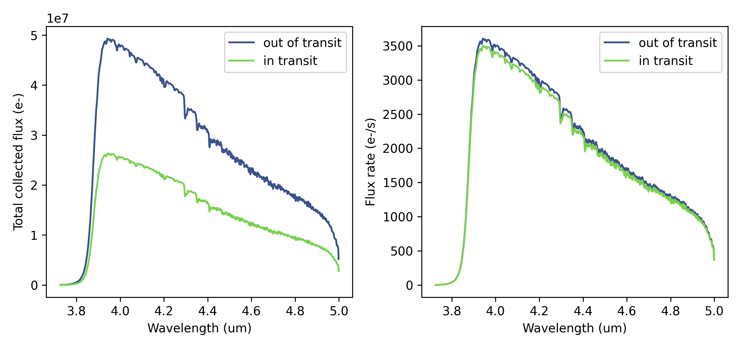
Save TSO outputs
The latest TSO run for a given Pandeia object can be saved with this method:
pando.save_tso(filename='tso_transit_WASP-80b_nircam_lw_f444w.picke')See this tutorial to load that pickle file and simulate some spectra.